- linking and dynamically displaying data...
Excel Pivot tables are an exceptionally powerful feature in Excel. They provide inbuilt functionality that allows data in spreadsheets to be quickly filtered, re-organised and managed based on set parameters.
This example will show how an Excel pivot table can be linked to data in an Access database.
You will normally need to import data from more than one table. For example, to get information about music shop CD sales you may need data from tables such as 'Salesman', 'Shop', and 'Sales' before you have enough data to make an analysis about sales patterns. One way to achieve this is to write a query in Access that gathers all the information you need from each table, then import the date from the Query to the Excel spreadsheet, and use a pivot table to display it. A second way is to use MSQuery when linking the Access database to the Excel spreadsheet. In this example the data exists in an external source, the Access database. If the tables relationships are established, then these will be included in the MSQuery design, but the relationships between tables can be amended before the data is imported to Excel.
The example will use Excel 2002 and then look at some of the differences when using Excel 2007.
- PivotTable Wizard & MSQuery...
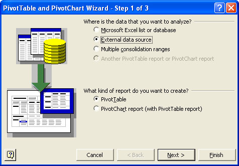
The process of gathering data to use in a pivot table begins by opening a worksheet where the data is to be displayed and then on the main menu choose Data>Pivot Table and Pivot Chart Report. This opens the Pivot Table and Pivot Chart Wizrd. In Step 1 choose External data source since we are using an Access database, and we want to create a Pivot Table.
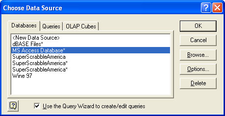
Step 2 is where you click the Get Data button. This opens MS Query. First, you must
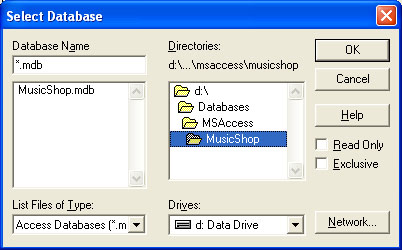
choose the data source, which in this example is MS Access Database. Then click the Browse button to find the Access database that contains the data.
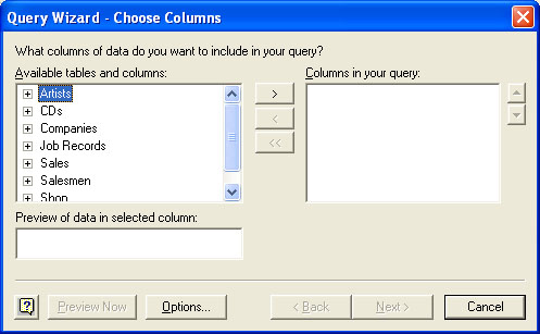
After selecting the database and clicking OK MS Query continues by displaying the available tables and columns. If there is a Query in your Access database then this will also be listed here. We shall assume that there are only tables to work from.
|
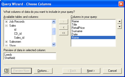
MS Query prompts you to add an arbitrary number of fields as 'Columns in your query' which is a little confusing. Lets consider that the data we are trying to obtain is CD sales by Salesman. We will need columns from the Artists, CDs, Sales, and Salesmen tables.
If there is already a relationship between these tables in MS Access then the data can be retrieved easily, although you should be careful to only include those columns you actually require.
If you ask for data that lives in two tables that are not related in the Access database you will be prompted to build the relationship at this point in the wizard. |
Here is the graphical representation of the tables in the MS Access database: 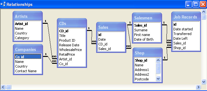 |
In extracting data about sales we will assume that the data needed includes: -
i) Name of Artist
ii) Title of CD
iii) Retail Price of CD
iv) Date sold
v) Salesman surname
vi) Shop name
The Artists, CDs, Sales and Salesmen tables are linked in the database, but there is no direct relationship to the Shop table from the Salesmen table. |
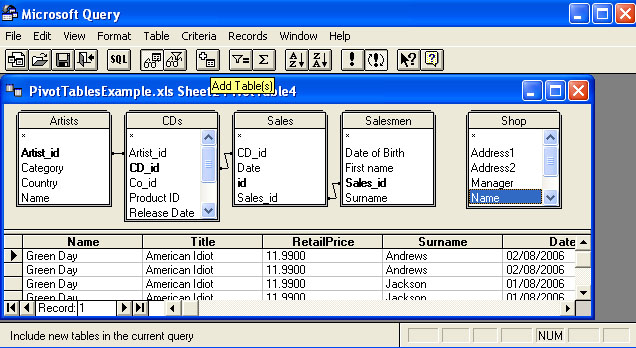
Lets assume that we exclude any data from the Job Records table when building the query. If teh JobRecords table is excluded, there is no link that MSQuery can build between the the Salesmen and Shop tables.
Therefore, MS Query warns you that there is no link between the tables.
Clicking OK will open a graphical display within MSQuery where you can click the Add Table button to add the JobRecords table and establish a link between the 5 tables. |
 |
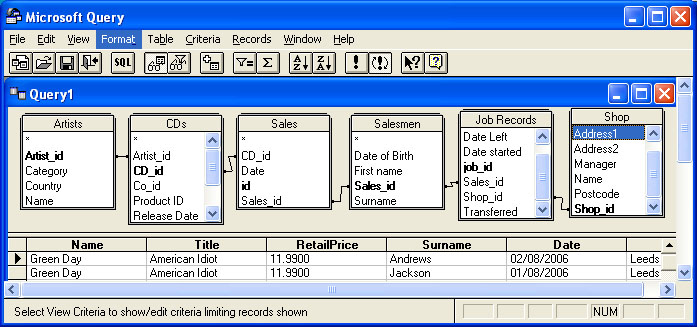
By adding the missing Job Records table a link is established between the Salesmen and Shop tables, allowing the data to be retreived from Access. Here are the columns that will be included in the query. We do not need any data from the Job Records table, we just need to use that table to establish the relationship. Clicking Next closes MS Query and brings us to Step 3 of the wizard, which includes the important Layout and Options buttons.
 |
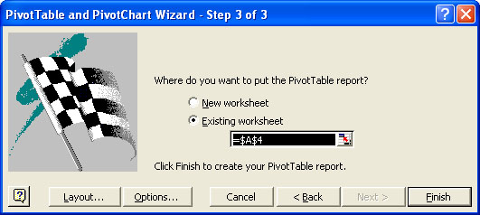
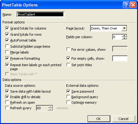
The Layout button is where the pivot table is contructed based on the available data, and the Options button allows you to make general changes to the formatting. |
|
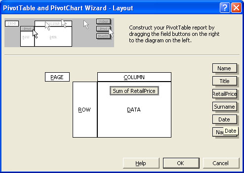
Clicking the layout Option opens the Layout dialog box. Lets assume the Reports output is the value of sales. The key data item is therefore RetailPrice. Use the mouse to drag the RetailPrice button from the right to the DATA section of the report. |
 |
|
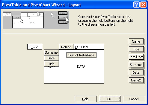
Drag Name2 (the Shop name) to the COLUMN area, and SURNAME, DATE & TITLE to the ROW area of the Layout diagram, as shown
Then click OK, and Finish to open the pivot table in Excel.
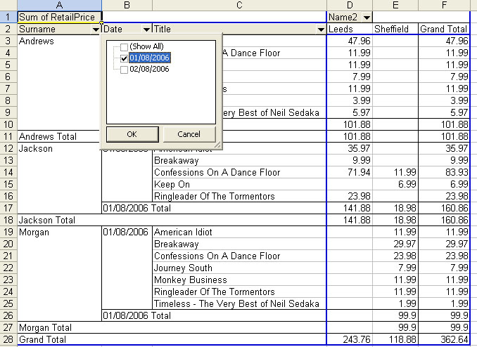
The image below shows the final Pivot Table. SURNAME DATE and TITLE are ROWS that are represented by buttons in row 2 of the spreadsheet. Here the Date button has been clicked and the pivot table has been filtered to only include sales for 01/08/2006.
Name2 is a COLUMN and is represented by the small button in column D. Both Leeds and Sheffield are represented in the pivot table at the moment. |
 |
| 
Additional options can be found by clicking the small buttons in the Layout section of the Pivot Table
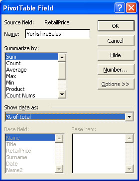
Double click the SumOfRetailPrice button in the layout Section, and a number of additional options become available, including a percentage field, and the ability to change the column heading in the Report,. in this example to "YorkshireSales".
The Options button allows the data item to be re-displayed as a percentage, in the pivot table. There are a number of other functions available, including using a running total, or a percentage difference from a particular item.
|
The completed Pivot Table. The data displayed can be easily filtered sing any of the column or row buttons. By clicking anywhere in the Pivot table and choosing Data>Pivot Table and Pivot Chart Report from the Excel top menu, you can easily change the fields included in the report. The Layout button gives additional options...
|
Here are some differences between using pivot tables in Excel 2007.
i) To create a pivot table you click on an Excel cell and use the Insert>Pivot table option on the main menu. If there is already a table of data Excel will highlight the table, you can edit the selected cells if the selection is inappropriate.
ii) To format data to include pound or dollar signs, or restrict to a number of decimal points, click any cell in the data column and choose Number Format
iii) To change the Sum to the average, click on the value in the bottom right and a dialog box appears enabling you to change from Sum to Average. You could add SumOfSales again, and change that one only to Average, to show both Sales volumes and averages on the same pivot table
iv) Formatting is available via the Design button, hovering the mouse automatically previews the pivot table design.
v) To show the top 5 values only, click the pivot table data area, and chose Filter, and Top 10, before changing the value to 5.
v) Once the pivot table is prepared, double clicking on any cell produces a sub-report for that item on a new worksheet.
vi) To add, minimum, maximum and average values, click the item that you want summarising, presumably one of the ROW values, choose Field Settings, then Custom, select the little box that allows more than one item and add Av, Max and Min.
|
| examples |
 |
|